CS229 Notes (Part 1): Mathematical Basics of Linear Regression — From Model Formulation to Gradient Descent

1. Introduction:
2. Linear Regression with One Variable

Introduction:

Welcome to the world of Machine Learning

Machine learning (ML) is one of the most exciting fields in modern computer science.
From natural language processing and spam filters to image recognition,computer vision, recommendation systems, self-driving cars, agriculture and medicine, machine learning is everywhere.

This course will not only cover cutting-edge theories of machine learning but also emphasize hands-on practice. By implementing algorithms yourself, you will gain a deep understanding of their internal mechanisms. This is crucial because merely mastering algorithms and mathematical knowledge is not sufficient to solve practical problems.

The popularity of machine learning stems from its ability to break the limitations of traditional programming. For complex tasks such as web search and photo tagging, we cannot directly write fixed programs to achieve the desired outcomes. Instead, machine learning enables computers to independently learn solutions from data. Today, machine learning is widely used in numerous fields including database mining, medical record analysis, computational biology, and unmanned helicopter control, with market demand far exceeding the supply of professionals.

Learning ML is not just about formulas and algorithms, but also about:

Understanding which problems are suitable for ML
Knowing how to choose models and methods
Being able to implement and tune algorithms in practice

What Is Machine Learning?

Two Classic Definitions:

1.Arthur Samuel (1950s):

The field of study that gives computers the ability to learn without being explicitly programmed.
He wrote a chess program that played against itself; through thousands of self-played games, the program surpassed its own creator.

2.Tom Mitchell (Modern):

A computer program is said to learn from experience E with respect to some class of tasks T and performance measure P, if its performance at tasks in T, as measured by P, improves with experience E.

Memory formula: T(E)ₚ - Improving task T’s performance on metric P through experience E

Example: Spam Filter

T (Task): Classify emails as spam or not spam
E (Experience): Samples marked as spam by users
P (Performance): Probability of correctly identifying spam emails

In simple terms:
👉 Instead of hard-coding rules, we let machines learn patterns from data.

Why machine learning?
Because for many complex problems:

❌ It is hard to write explicit rules
✅ But we often have plenty of data to learn from

Supervised Learning

Supervised learning means that each sample in the training dataset is accompanied by a “correct answer” (label). The algorithm learns the mapping relationship between sample features and labels to achieve prediction for new samples.

Characteristics:

Training data include inputs x and correct outputs y
The goal is to learn a mapping from x → y

Form:
(x, y)

Two main types:

✅ Regression Problems - Predicting continuous values
such as:

House prices
Temperature

Sales

Example: House price prediction
Input: House area (750 square feet)
Output: Predicted price ($150,000)
Feature: Output is continuous numerical values that can take any real number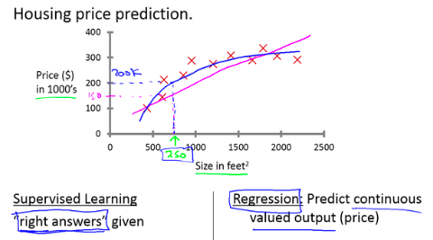

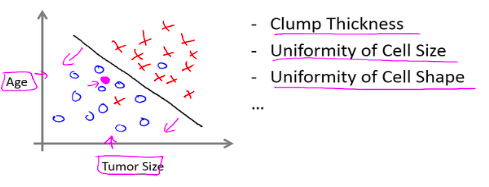
✅ Classification Problems - Predicting discrete categories

such as:

Spam / not spam
Disease / healthy

Image categories

Example: Tumor diagnosis
Input: Tumor features (size, density, etc.)
Output: Benign(0) / Malignant(1)
Feature: Output is a finite set of discrete values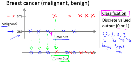

Essence of supervised learning:

Learn from labeled data so the model can make predictions on new examples.

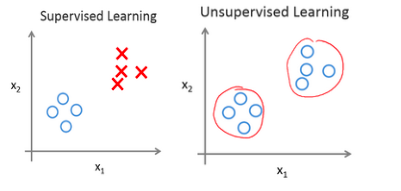
Unsupervised Learning

The core difference between unsupervised learning and supervised learning is that training data has no labels. The algorithm needs to independently discover potential structures from the data. A typical representative of unsupervised learning is clustering algorithms.

Characteristics:

Only input data x
No labels y
The goal is to discover structure in the data

Common task: Clustering

Applications:

Automatically grouping news (e.g., Google News)
Customer segmentation
Gene analysis
Community detection in social networks

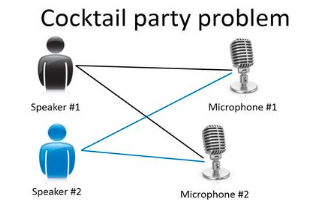
Cocktail Party Problem:

matlab:

1 2	% Audio separation achieved with just one line of code [W,s,v] = svd((repmat(sum(x.x,1),size(x,1),1).x)*x');

Separating different speakers’ audio from mixed sounds
Demonstrates the importance of using the right tools

Intuition:

We do not know the categories in advance, but want the algorithm to find similar groups by itself.

Comparison:

Size in feet	Labeled?	Goal
Supervised Learning	Yes	Prediction
Unsupervised Learning	No	Discover structure

Linear Regression with One Variable

Model Representation

Linear regression with one variable is an introductory machine learning algorithm used to solve single-feature regression problems (e.g., predicting house prices using house size).
Let’s start with an example: This example is about predicting house prices, and we’ll use a dataset containing housing prices in Portland, Oregon. Here, I’ll plot our dataset based on the prices of houses sold for different house sizes.
For instance, if your friend’s house is 1,250 square feet in size, you want to tell them how much it could sell for. One thing you can do is build a model—perhaps a straight line—and from this model, you might tell your friend they could sell the house for about $220,000.
This is an example of a supervised learning algorithm.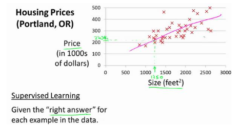

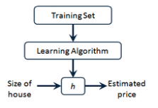
Training Set: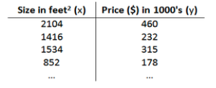

Notation:

m: number of training examples
x: feature
y: target
(x⁽ⁱ⁾, y⁽ⁱ⁾): The i-th training example
h(x): hypothesis (model),used to predict the value of y
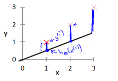
Univariate linear regression model:
1
hθ(x) = θ₀ + θ₁ x

This is a straight line, where:

θ₀ is the intercept,the point where the hypothesis function intersects the y-axis
θ₁ is the slope,the degree of influence of feature x on target y

Goal:
Find θ₀ and θ₁ so that the line fits the data as well as possible.

Cost Function

To measure the prediction error of the hypothesis function, we need to define a Cost Function, which primarily calculates the sum of squared errors between predicted values and actual values.

Definition of the Cost Function

Linear regression with one variable uses the Mean Squared Error (MSE) as its cost function, defined by the formula:

1	J(θ₀, θ₁) = (1 / 2m) * Σ (hθ(x⁽ⁱ⁾) - y⁽ⁱ⁾)²

1/2: Included to cancel out the coefficient from the square term during differentiation, simplifying calculations
Σ (hθ(x⁽ⁱ⁾) - y⁽ⁱ⁾)²:Sum of squared prediction errors for all samples
J(θ₀, θ₁)： A smaller value of the cost function indicates higher prediction accuracy of the model

Meaning:
Square the errors
Average over all training examples
The smaller, the better

👉 Our objective:

1	minimize J(θ₀, θ₁)

Why Choose Squared Error?

Mathematically: Facilitates differentiation and enables smoother optimization
This is the primary reason.

The squared function (y-ŷ)² is a smooth convex function everywhere, and its derivative is 2(y-ŷ), which is very simple.
The absolute function |y-ŷ| is not differentiable at y=ŷ (it has a “sharp point”). This can cause gradient‑based optimization algorithms like gradient descent to get “stuck” at that point and require special handling.

An intuitive analogy:
Squared error is like a smooth, bowl‑shaped curve—a ball (the optimization process) can roll smoothly down to the bottom of the bowl (the minimum).
Absolute error is like a folded V‑shaped piece of paper with a sharp crease—when the ball reaches the tip, it gets stuck and doesn’t know which way to roll.

Statistically: Aligns with the assumption of maximum likelihood estimation
When we assume that data errors follow a normal (Gaussian) distribution, maximizing the likelihood function is equivalent to minimizing the mean‑squared error. This is the statistical foundation of many linear models. Since the normal distribution is common in nature, this assumption is often reasonable.
In terms of effect: Penalizes large errors more heavily, making it more sensitive to outliers
Error² amplifies the impact of large errors.

Advantage: The model will try hard to avoid large prediction mistakes, because the cost grows quadratically with the error. This is usually what we want.
Disadvantage: If there are outliers in the data, squaring magnifies their influence, which can “pull” the model off course. (In such cases, absolute error or Huber loss can be used to mitigate the issue.)

Example:
Error = 1 → squared cost = 1
Error = 2 → squared cost = 4 (4 times the cost for 2 times the error)
Error = 10 → squared cost = 100 (100 times the cost for 10 times the error)

Good mathematical properties (convex function, has unique minimum)
Heavily penalizes large errors
Performs well in practical applications

Intuition for the Cost Function (I)

Imagine different lines:

Some are far from the data → large error → large J
Some fit the data well → small error → small J

So J tells us:
👉 On average, how badly this line fits the data.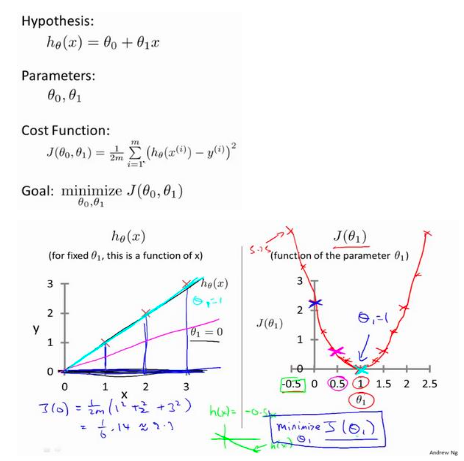

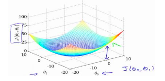
Intuition for the Cost Function (II): Contour Plots

If we treat θ₀ and θ₁ as axes, and J(θ₀, θ₁) as height:

We get a bowl-shaped surface
The lowest point corresponds to the best parameters

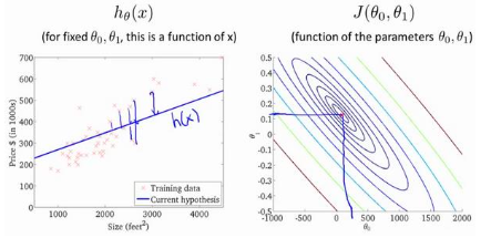
A contour plot shows:

Each closed curve has the same J value
Inner curves mean smaller J

👉 Learning is like:
Going downhill on an error landscape until we reach the bottom.

Gradient Descent

Gradient descent is a general algorithm for minimizing functions.

Core Idea:

Starting from a random point, take small steps along the steepest downhill direction until reaching the valley bottom

Step:

Start from some initial point (θ₀, θ₁)
Take a small step in the direction of steepest decrease of J

Repeat until convergence
Update rule:

1	θⱼ := θⱼ - α * ∂J(θ) / ∂θⱼ

Where:

α is the learning rate (step size)
:= Denotes assignment, meaning the value on the right-hand side is computed first to update the parameter on the left-hand side

👉 Analogy:
Walking downhill while blindfolded, always stepping in the steepest direction.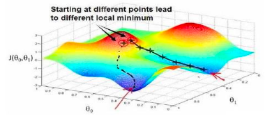

Gradient Descent Intuition

The core of gradient descent lies in the coordination between the learning rate α and the gradient direction, which can be intuitively understood using a single-parameter example:

Role of the Gradient

When the gradient is positive: θⱼ decreases (θⱼ := θⱼ − α × positive number),causing the cost function to decrease
When the gradient is negative: θⱼ increases (θⱼ := θⱼ − α × negative number)causing the cost function to decrease
When the gradient is zero: θⱼ stops updating, indicating that the minimum point has been reached

Impact of Learning Rate α

α too small: Small parameter update steps result in slow convergence, requiring numerous iterations to reach the minimum point
α too large: May overshoot the minimum point, causing the cost function to diverge and fail to converge
Adaptive Convergence: As parameters approach the minimum point, the gradient gradually decreases. Even with a fixed α
, the magnitude of parameter updates automatically becomes smaller, leading to eventual convergence.

Gradient Descent for Linear Regression

Combining the gradient descent algorithm with the linear regression cost function yields the gradient descent solution for linear regression.

Calculating Partial Derivatives

Compute the partial derivatives of the linear regression cost function $J(\theta_0, \theta_1)$:

Partial derivative with respect to $\theta_0$:

1	∂/∂θ₀ J(θ₀, θ₁) = (1/m) * Σⁱ₌₁ᵐ (h_θ(x⁽ⁱ⁾) - y⁽ⁱ⁾)

Partial derivative with respect to $\theta_1$:

1	∂/∂θ₁ J(θ₀, θ₁) = (1/m) * Σⁱ₌₁ᵐ (h_θ(x⁽ⁱ⁾) - y⁽ⁱ⁾) · x⁽ⁱ⁾

Gradient Descent Update Rule for Linear Regression

Substitute the partial derivatives into the gradient descent formula to obtain:

1
2
3

θ₀ := θ₀ - α · (1/m) * Σⁱ₌₁ᵐ (h_θ(x⁽ⁱ⁾) - y⁽ⁱ⁾)

θ₁ := θ₁ - α · (1/m) * Σⁱ₌₁ᵐ (h_θ(x⁽ⁱ⁾) - y⁽ⁱ⁾) · x⁽ⁱ⁾

Summary of the Algorithm Process

Initialize parameters θ₀ and θ₁ (e.g., set both to 0)
Compute the prediction errors h_θ(x⁽ⁱ⁾) - y⁽ⁱ⁾ for all training samples
Substitute into the update rule to simultaneously update θ₀ and θ₁
Repeat steps 2-3 until the change in the cost function J(θ₀, θ₁) is smaller than a threshold value (convergence)
Output the optimal parameters θ₀ and θ₁ to obtain the final hypothesis function

Supplement: Batch Gradient Descent vs. Normal Equation

Batch Gradient Descent: Suitable for large datasets, solves the problem iteratively and requires selecting a learning rate
α
Normal Equation: Solves for the optimal parameters directly through matrix operations without iteration or learning rate selection. However, it has high computational complexity and is suitable for small datasets